SIGMA's BLOG

但行好事,莫问前程

卷积操作

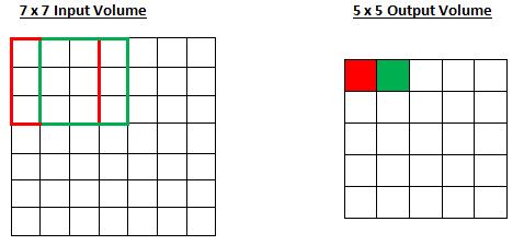
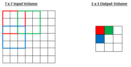
$O$是output_shape,$W$是image,$K$是filter,$P$是padding,$S$是stride

stride = 1

stride = 2

Padding

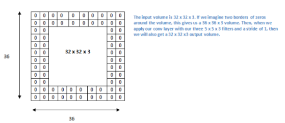
  • padding的计算公式与conv一样
  • zero padding

有这些情况会使用zero padding

  • 卷积后image尺寸很小,但我们又想使用conv
  • 由于image尺寸跟filter尺寸的原因

pooling

也叫downsampling(下采样)层,最常用的是max-pooling

stride = 2

ReLu

优点:

  • 因为它在准确度不发生明显改变的情况下能把训练速度提高很多
  • 能够减轻vanishing gradient problem
    —指梯度以指数方式在层中消失,导致网络较底层的训练速度非常慢
  • 把negative activation变为0,增加了模型的非线性特征,而且不影响感受域

参见 Geoffrey Hinton(即深度学习之父)的论文:Rectified Linear Units Improve Restricted Boltzmann Machines

Dropout

随机丢弃神经元,简单来说,就是在训练过程中在Dropout层设置一个随机的激活参数集,在forward pass中将这些激活参数集设置为0。

理解了大概,这部分细节需要详细看看

参考资料
https://www.zhihu.com/question/52668301

Intro

本文记录了阅读论文Dynamic Routing Between Capsules以及naturomics的代码的理解与收获,若有错误欢迎指出(wjy.f@qq.com),转载请注明出处。

若想通过视频快速了解,可以看看下面两个链接,讲得比较生动易理解(不过还是推荐读论文):


Main

CapsNet

结构概述

论文仅仅是提出了一个可行的方案,目的是为了证明Capsule这个思想的可行性,目前还较为粗略,有很多改进空间。论文有两个比较突出的创新点:

  • 采用 routing-by-agreement mechainsm 决定两层capsule之间的连接以及参数$c_{ij}$的更新方式
  • 用向量输出替代标量输出

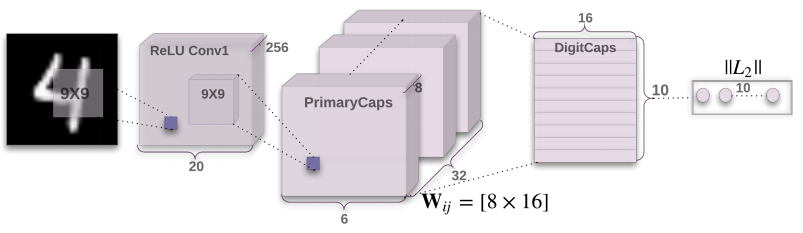
下图是论文中所采用的神经网络结构:

看完这幅图应该大概能理解CapsNet的结构。它先是对图像用了两次卷积得到PrimaryCaps,然后用Routing-By-Agreement Mechanism得到DigitCaps。最后,求DigitCaps中的10个向量的长度,比如说最长的是第4个向量,那么就意味着CapsNet识别出当前输入的图片是数字4。

看到这里,何为Capsule?在PrimaryCaps中,它指的是长度为8的向量,共6632个。而在DigitCaps中,它指的是16维的向量,共10个。所以Capsule其实对应着传统神经网络的scalar,只是一个scalar能够表征的信息太少了,所以将其扩展为向量,这样它就能够表示更多的信息。有人说,之所以提出这种想法是因为Hinton观察到人的大脑不是像神经网络一样严格分层,而是一簇簇神经元作为一个整体的。

CapsNet的结构是Image(input)->Conv1->PrimaryCaps->DigitCaps(output)->Reconstruction,下文也会按照这个顺序来讲解

在下文中,若 i 指 $layer_l$ 的某一个capsule ,那么 j 就是指 $layer_{l+1}$ 的某一个capsule。

image to ReLU Conv1 to PrimaryCaps

论文使用的是MNIST手写识别数据集,每张图片的大小都是28*28。

流程:

  1. image(28 * 28)

  2. images $\to$ Conv(num_outputs=256, kernel_size=9, stride=1, padding='VALID') + ReLU $\to$ Conv1(256*20*20)

  3. Conv1 $\to$ Conv(num_outputs=256, kernel_size=9, stride=2, padding="VALID") + ReLU $\to$ PrimaryCaps(256*6*6)

这里可能会有人奇怪,这里不过是用了256个filter产生256个feature map,图片为什么会画成(32*8*6*6)的形式,这是因为后面的路由算法是将一个长度为8的向量当做一个整体来计算的。

PrimaryCaps to DigitCaps & Dynamic Routing

  • 下面讲解从PrimaryCaps $\to$ DigitCaps的计算过程,其中主要应用了Routing-By-Agreement Mechanism

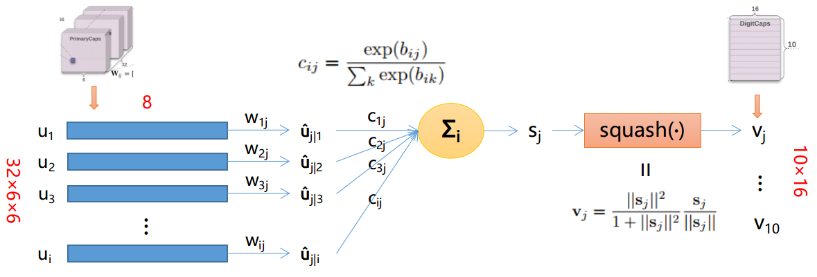
一张图表示他们之间的关系:

注意,图片中仅展示了一个$v_j,j\in(1,10)$的求解过程,其他$v_j$同理可得。

公式

  • $u_i(i \in [6 × 6 × 32])$: 表示PrimaryCaps的某个8D的Capsule
  • $\hat{u}_{j|i}$: 论文中称之为低一层的capsules的“prediction vectors”
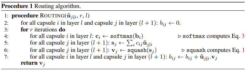
  • $b_{ij}$: 初始化为0,更新方法是 $b_{ij} \leftarrow b_{ij} + \hat{u}_{j|i} v_j$。 其中$a_{ij} = \hat{u}_{j|i} v_j$表示$capsule_j$(即$v_j$)跟$capsule_i$的prediction vector(即$\hat{u}_{j|i}$)的agreement(契合度)。值越大,表示两个向量的方向越相似,两个向量所表示的性质越相近。由 $c_{ij}$ 的公式知,$b_{ij}$ 的值越大(意味着两个向量的方向越相似),$c_{ij}$ 的值越大,$capsule_i$ 越倾向于将信息传送给 $capsule_j$
  • $c_{ij}$: 由动态路由算法更新的coupling coefficients,并且 $\sum{i} c\{ij} = 1$(此时$j$为某确定的常数)
  • $s_j$: $capsule_j$ 的所有input之和。
  • $squash()$: 非线性函数,保留了向量的方向,使长的向量越长,短的向量越短,并且长度都压缩在0-1之内
  • $v_j$: 由dynamic routing计算出来的PrimaryCaps的output。在文章中就是指最后的输出DigitCaps,共有10个(因为有10个数字,即10类)Capsule。每个capsule有16维,每一维都代表着数字的某些属性(粗细、倾斜程度等等)。向量的长度代表了当前输入是类 $j$ 的概率

Dynamic Routing算法流程

整个过程如下所示(图片来自naturomics的ppt):

Reconstruction

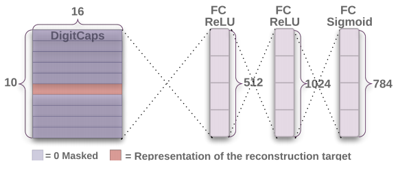
CapsNet使用Reconstruction作为Regularization。其做法是将DigitCaps的十个输出向量$v_j$中长度最长的向量,经过3个FC层(结构如下图所示)重构出原来的图像,通过对比重构的图像和原图像的差异(pixel-wise),得到reconstruction loss。用来重构的这三个FC层一起称为Decoder

Total loss

由于有多个类的存在,所以不能用cross entropy,论文中使用了SVM中常用的损失函数Margin loss来代替

Margin loss

  • k: class k,$k\in[1, 10]$
  • $m^+=0.9, m^-=0.1$ (自己设定)
  • $\lambda$ (比例系数,用来调整两者的比重):

    The λ down-weighting of the loss for absent digit classes stops the initial learning from shrinking the lengths of the activity vectors of all the digit capsules. We use λ = 0.5.

  • 如果输入的数字图像是class k,那么$T_k=1$

  • | 示例 | 输入输出 | $|v_k|$ | $L_k$ |
    | — | ——————————- | ——- | ——- |
    | TT | 输入数字k 预测结果为数字k | 比较大 | 比较小 |
    | TF | 输入数字k 预测结果非数字k | 比较小 | 比较大 |
    | FT | 输入非数字k 预测结果为数字k | 比较大 | 比较大 |
    | FF | 输入非数字k 预测结果非数字k | 比较小 | 比较小 |
  • 可以看出,在假阳性和假阴性的示例中,$L_k$的值比较大。

Reconstruction loss

计算原图像与重构的图像在对应的pixel位置上的值之差,求和得到Reconstruction loss

1
2
3
4
将原图像x(28, 28)reshape成orgin(784)
再将重构的图像decoded(784)
squared = square(decoded - orgin)
reconstruction_loss = mean(squared)

最后:


实验

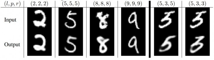
MNIST

l=label, p=prediction, r=reconstruction。下面最右的两列展示了模式是如何在5和3之间纠结的。而其它列表明了模型不仅保留了图片的细节并且平滑了噪声。

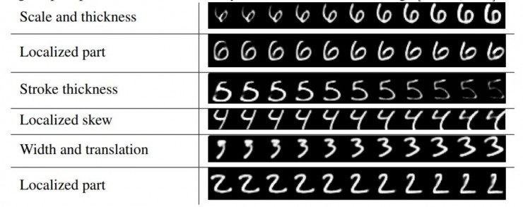
Dimension perturbations

改变DigitCaps中的capsule的16维中的一维,这个被改变的capsule所重构出来的图像也会有所变化(比如笔画变得更粗)。这表明了capsule学习到了entity,并且每一维都代表着entity的某个feature,具有很强的解释性。

MultiMNIST

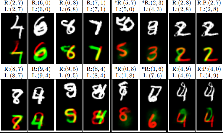
L指的是两个label,R指的是两个用于重构的图像。上面白色的是input image,下面红绿色重叠的是重构的图像。

如下图所示,实验把两个激活程度最高的capsule对应的数字作为识别结果,据此对识别到的图像元素进行了重构。对于左边中识别正确的样本(L指真实标签,R指激活程度最高的两个胶囊对应的标签),可以看到由于不同的capsule各自工作,在一个识别结果中用到的特征并不会影响到另一个识别结果,不受重叠的影响(或者说重叠部分的特征可以复用)。

另一方面,每个capsule还是需要足够多的周边信息支持,而不是一味地认为重叠部分的特征就需要复用。下图中间是选了一个高激活程度的capsule和一个低激活程度capsule的结果(* R表示其中一个数字既不是真实标签也不是识别结果,L仍然为真实标签)。可以看到,在(5,0)图中,关注“7”的capsule并没有找到足够多的“7”的特征,所以激活很弱;(1,8)图中也是因为没有“0”的支持特征,所以重叠的部分也没有在“0”的capsule中用第二次。

最右R:P:(2, 7)指的是预测结果是2,7,然后将代表2和7的capsule重构。


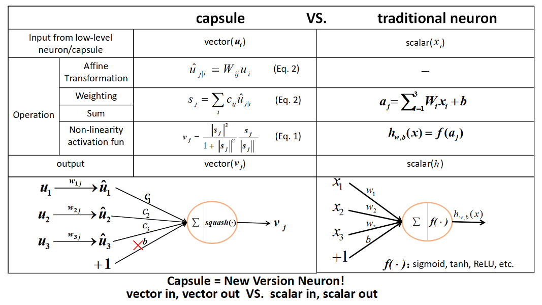
CapsNet与tradictional neuron的对比

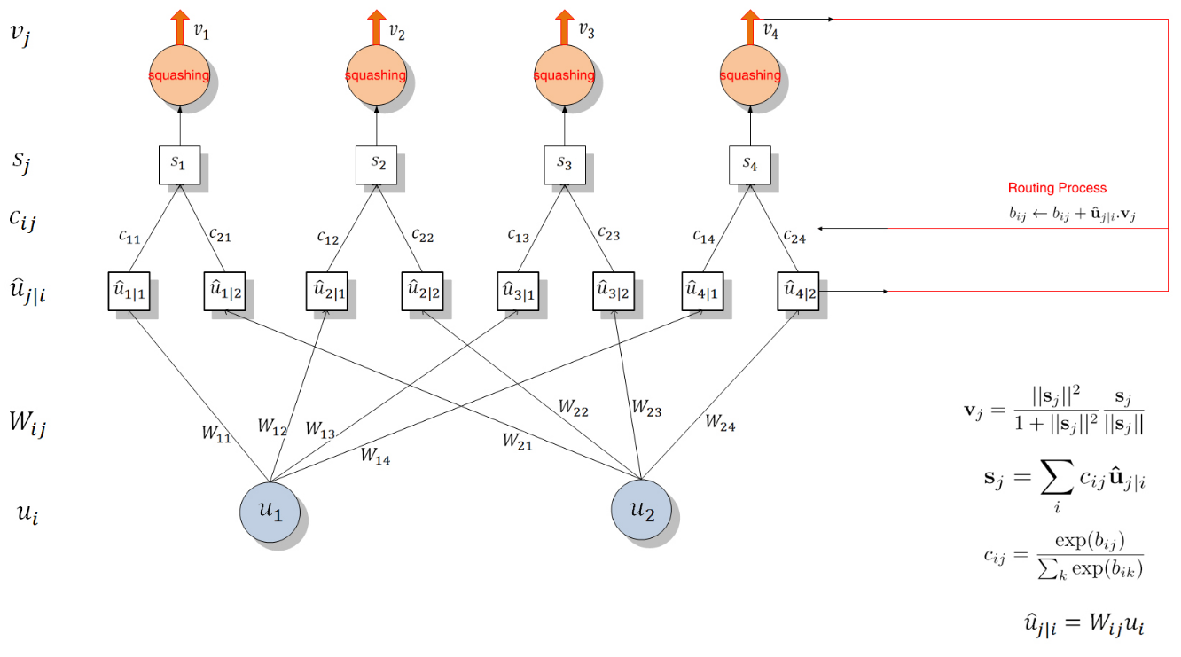
(图片来自naturomics):


总结

为什么要用Routing-by-agreement?

传统的CNN里面,conv后面是max-pooling层,但是max-pooling只保留了唯一一个最活跃的特征,而Routing则有效得多。

Routing-by-agreement有以下几个好处:

  • 由于上一层的capsule会逐渐倾向于将信息传到下一层与它相似的capsule,这样就能够给下一层capsule干净清晰的信号,减少噪声,从而更快地学习到entity
  • 通过追溯当前被激活的capsule的信号传输路径,我们可以操控part-whole中的part,并且清楚知道哪一个part属于哪一个entity(比如说识别一个由三角形和长方形组成的房屋,在$layer l$可能有个capsule是检测三角形,有个capsule检测长方形,则在$layer l+1$有能够得到检测房屋的capsule。此为ppart-whole的关系)。
  • 可以很容易地解析重叠的entity,比如重叠的数字识别。

the capsules in the first layer try to predict what the second layer capsules will output


代码阅读

代码link

由于代码基本上都是按照文章思路来写的,所以不重复讲,而是介绍主要的结构。

目录

1
2
3
4
5
6
7
8
9
10
11
12
13
14
15
16
17
18
19
20
21
22
23
24
25
CapsNet-Tensorflow
- capsLayer.py
定义了capsLayer的实现方法。
由于论文中提及的capsLayer有两种:
PrimaryCaps(without routing)
DigitCaps(with routing)
所以该文件里面也包含了这两种Layer的实现方式
另外,该文件还有:
routing
squash

- capsNet.py
定义了CapsNet类
包含:
build_arch() # 定义结构
loss() # 定义loss

- config.py
超参数设定

- main.py
程序入口

- utils.py
用于读取MNIST的数据

主要代码:

1
2
3
4
5
6
7
8
9
10
11
12
13
14
15
16
17
18
19
20
21
22
23
24
25
26
27
28
29
30
31
32
33
34
35
36
37
38
39
40
41
42
43
44
45
46
47
48
49
50
51
52
53
54
55
56
57
58
59
60
61
62
63
64
65
66
67
68
69
70
71
72
73
74
75
76
77
78
79
80
81
82
83
84
85
86
87
88
89
90
91
92
93
94
95
96
97
98
99
100
101
102
103
104
105
106
107
108
109
110
111
112
113
114
115
116
117
118
119
120
121
122
123
124
class CapsNet(object):
def __init__(self, is_training=True):
self.graph = tf.Graph()
with self.graph.as_default():
if is_training: # 如果是在训练过程中
self.X, self.labels = get_batch_data() # 获取training data和label
self.Y = tf.one_hot(self.labels, depth=10, axis=1, dtype=tf.float32) # 对label做onehot

self.build_arch() # 搭建CapsNet的结构
self.loss() # 定义loss
self._summary()

# t_vars = tf.trainable_variables()
self.global_step = tf.Variable(0, name='global_step', trainable=False)
self.optimizer = tf.train.AdamOptimizer() # 使用AdamOptimizer
self.train_op = self.optimizer.minimize(self.total_loss, global_step=self.global_step) # var_list=t_vars)
elif cfg.mask_with_y: # 如果是已经训练完
self.X = tf.placeholder(tf.float32,
shape=(cfg.batch_size, 28, 28, 1))
self.Y = tf.placeholder(tf.float32, shape=(cfg.batch_size, 10, 1))
self.build_arch()
else:
self.X = tf.placeholder(tf.float32,
shape=(cfg.batch_size, 28, 28, 1))
self.build_arch()

tf.logging.info('Seting up the main structure')

def build_arch(self):
with tf.variable_scope('Conv1_layer'):
# Conv1, [batch_size, 20, 20, 256]
conv1 = tf.contrib.layers.conv2d(self.X, num_outputs=256,
kernel_size=9, stride=1,
padding='VALID')
assert conv1.get_shape() == [cfg.batch_size, 20, 20, 256]

# Primary Capsules layer, return [batch_size, 1152, 8, 1]
with tf.variable_scope('PrimaryCaps_layer'):
primaryCaps = CapsLayer(num_outputs=32, vec_len=8, with_routing=False, layer_type='CONV')
caps1 = primaryCaps(conv1, kernel_size=9, stride=2)
assert caps1.get_shape() == [cfg.batch_size, 1152, 8, 1]

# DigitCaps layer, return [batch_size, 10, 16, 1]
with tf.variable_scope('DigitCaps_layer'):
digitCaps = CapsLayer(num_outputs=10, vec_len=16, with_routing=True, layer_type='FC')
self.caps2 = digitCaps(caps1)

# Decoder structure in Fig. 2
# 1. Do masking, how:
with tf.variable_scope('Masking'):
# a). calc ||v_c||, then do softmax(||v_c||)
# [batch_size, 10, 16, 1] => [batch_size, 10, 1, 1]
self.v_length = tf.sqrt(tf.reduce_sum(tf.square(self.caps2),
axis=2, keep_dims=True) + epsilon)
self.softmax_v = tf.nn.softmax(self.v_length, dim=1)
assert self.softmax_v.get_shape() == [cfg.batch_size, 10, 1, 1]

# b). pick out the index of max softmax val of the 10 caps
# [batch_size, 10, 1, 1] => [batch_size] (index)
self.argmax_idx = tf.to_int32(tf.argmax(self.softmax_v, axis=1))
assert self.argmax_idx.get_shape() == [cfg.batch_size, 1, 1]
self.argmax_idx = tf.reshape(self.argmax_idx, shape=(cfg.batch_size, ))

# Method 1.
if not cfg.mask_with_y:
# c). indexing
# It's not easy to understand the indexing process with argmax_idx
# as we are 3-dim animal
masked_v = []
for batch_size in range(cfg.batch_size):
v = self.caps2[batch_size][self.argmax_idx[batch_size], :]
masked_v.append(tf.reshape(v, shape=(1, 1, 16, 1)))

self.masked_v = tf.concat(masked_v, axis=0)
assert self.masked_v.get_shape() == [cfg.batch_size, 1, 16, 1]
# Method 2. masking with true label, default mode
else:
# self.masked_v = tf.matmul(tf.squeeze(self.caps2), tf.reshape(self.Y, (-1, 10, 1)), transpose_a=True)
self.masked_v = tf.multiply(tf.squeeze(self.caps2), tf.reshape(self.Y, (-1, 10, 1)))
self.v_length = tf.sqrt(tf.reduce_sum(tf.square(self.caps2), axis=2, keep_dims=True) + epsilon)

# 2. Reconstructe the MNIST images with 3 FC layers
# [batch_size, 1, 16, 1] => [batch_size, 16] => [batch_size, 512]
with tf.variable_scope('Decoder'):
vector_j = tf.reshape(self.masked_v, shape=(cfg.batch_size, -1))
fc1 = tf.contrib.layers.fully_connected(vector_j, num_outputs=512)
assert fc1.get_shape() == [cfg.batch_size, 512]
fc2 = tf.contrib.layers.fully_connected(fc1, num_outputs=1024)
assert fc2.get_shape() == [cfg.batch_size, 1024]
self.decoded = tf.contrib.layers.fully_connected(fc2, num_outputs=784, activation_fn=tf.sigmoid)

def loss(self):
# 1. The margin loss

# [batch_size, 10, 1, 1]
# max_l = max(0, m_plus-||v_c||)^2
max_l = tf.square(tf.maximum(0., cfg.m_plus - self.v_length))
# max_r = max(0, ||v_c||-m_minus)^2
max_r = tf.square(tf.maximum(0., self.v_length - cfg.m_minus))
assert max_l.get_shape() == [cfg.batch_size, 10, 1, 1]

# reshape: [batch_size, 10, 1, 1] => [batch_size, 10]
max_l = tf.reshape(max_l, shape=(cfg.batch_size, -1))
max_r = tf.reshape(max_r, shape=(cfg.batch_size, -1))

# calc T_c: [batch_size, 10]
# T_c = Y, is my understanding correct? Try it.
T_c = self.Y
# [batch_size, 10], element-wise multiply
L_c = T_c * max_l + cfg.lambda_val * (1 - T_c) * max_r

self.margin_loss = tf.reduce_mean(tf.reduce_sum(L_c, axis=1))

# 2. The reconstruction loss
orgin = tf.reshape(self.X, shape=(cfg.batch_size, -1))
squared = tf.square(self.decoded - orgin)
self.reconstruction_err = tf.reduce_mean(squared)

# 3. Total loss
# The paper uses sum of squared error as reconstruction error, but we
# have used reduce_mean in `# 2 The reconstruction loss` to calculate
# mean squared error. In order to keep in line with the paper,the
# regularization scale should be 0.0005*784=0.392
self.total_loss = self.margin_loss + cfg.regularization_scale * self.reconstruction_err

概念

转自这里

什么是掩膜(mask)

数字图像处理中的掩膜的概念是借鉴于PCB制版的过程,在半导体制造中,许多芯片工艺步骤采用光刻技术,用于这些步骤的图形“底片”称为掩膜(也称作“掩模”),其作用是:在硅片上选定的区域中对一个不透明的图形模板遮盖,继而下面的腐蚀或扩散将只影响选定的区域以外的区域。

图像掩膜与其类似,用选定的图像、图形或物体,对处理的图像(全部或局部)进行遮挡,来控制图像处理的区域或处理过程。
光学图像处理中,掩模可以是胶片、滤光片等。数字图像处理中,掩模为二维矩阵数组,有时也用多值图像。数字图像处理中,图像掩模主要用于:

①提取感兴趣区,用预先制作的感兴趣区掩模与待处理图像相乘,得到感兴趣区图像,感兴趣区内图像值保持不变,而区外图像值都为0。
②屏蔽作用,用掩模对图像上某些区域作屏蔽,使其不参加处理或不参加处理参数的计算,或仅对屏蔽区作处理或统计。
③结构特征提取,用相似性变量或图像匹配方法检测和提取图像中与掩模相似的结构特征。
④特殊形状图像的制作。

掩膜是一种图像滤镜的模板,实用掩膜经常处理的是遥感图像。当提取道路或者河流,或者房屋时,通过一个n*n的矩阵来对图像进行像素过滤,然后将我们需要的地物或者标志突出显示出来。这个矩阵就是一种掩膜。

实例

简单例子见这里

进一步的例子还有这里

question

  • translation invariance是指什么,有什么作用
  • 其中一种loss:IoU —— Intersection of Union
  • Ground Truth
    -

3.

convnet = h w d (height, width, color channel)

基于translation invariance


三种技术

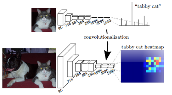
  • 卷积化(Convolutional)
  • 上采样(Upsample)
  • 跳跃结构(Skip Layer)

卷积化

FC换成Conv以保留图像的空间信息


上采样

此处的上采样即是反卷积(Deconvolution)。当然关于这个名字不同框架不同,Caffe和Kera里叫Deconvolution,而tensorflow里叫conv_transpose。CS231n这门课中说,叫conv_transpose更为合适。


Loss

对于最终输出的每一个像素的类别信息,我们并不把所有的像素点的结果计算到loss中进行反向传播,而是只取其中一部分的像素点。这个想法是有点道理的,因为每一个紧密相邻的像素点之前的特征差距可能并不大,如果每一个像素点都计算在内,那么就相当于我们对某一组特征增加了很高的权重。但好在我们对所有像素点都增加权重的话,这个影响还是会抵消的。

Why RNN

某些任务是需要NN具有记忆的,比如

  • 我 来了 台北
  • 我 离开了 台北

要确定我要离开还是来了台北,需要知道前一个单词是什么。这就需要网络具有记忆,于是就提出了RNN。

Why RNN’s error surface so rough

这是长距离传输引起的。假设有一个RNN,它的 memory 等于上一个时刻的 memory * w。除了第一个时刻 input = 1 之外,其他所有时刻 input = 0。那么在经过1001个时刻的传输后:

可以看到,w发生微小的变化会引起蝴蝶效应。这是长距离传输里面存在的问题,也是 error surface 抖动如此大的原因所在。

当然,这是李宏毅视频里面说的,我的问题是,这明显是一个单调函数,如何会引起剧烈抖动?

可能跟 training 过程中参数的微小变化有关。但是参数存在以下变动情况:

  • 参数经常有微小变化。这个应该不会形成蝴蝶效应吧?
  • 参数单调增减一段时间又单调减增。不明。
  • 参数总体是单调的。这种情况应该是逐渐变化的,不会出现剧烈抖动吧?
  • 参数经常剧烈变化,即 Gradient 值突然很大。根据前面视频的内容,RNN应该就是这种情况。只是如果是这种情况,他举上面那个长距离传输例子既不是都不相关了吗?

后来我通过编程发现,result *= w这种运算一开始 result(t)-result(t-1)只有0.几,但是到后面就有100+。

所以,这确实是原因所在,训练越到后面,Gradient 的值变化越来越大,error surface 的动荡越频繁越明显。所以作者想了下面的解决办法。

how to solve

由于RNN的 error surface 太陡峭,所以训练的时候有个技巧,就是当 Gradient 超过某个 threshold 的时候就不要让它超过那个 threshold 。比如说超过了15,就让它 = 15。这样,参数的变化就会相对不会起飞太严重。

RNN的training trick

Identity matrix + ReLU

对于一般的RNN来说,可以用单位矩阵+ReLU来初始化RNN,会有很好的效果


LSTM

具体实现用到的技巧

假设它的三个 GATE 的输入都是线性的,例如对 input-gate 来说,y = a1x1+a2x2+a3x3+a4b。它可以通过令 a4 = -10 来使 input-gate 有一定的阈值。

LSTM trick


GRU

如果发现LSTM过拟合很严重,可以试试这个。


Gradient vanished

提到上面的问题顺便提下 Gradient vanished

是 sigmoid 导致的。因为 sigmoid 的值在 [0, 1] 之间,所以在很深的网络里面会使每次的值越来越小,从而出现 vanished。

其实,Rough 和 Vanished 本质上都是长距离传输导致的问题。

在统计学里面,Huber loss是一个在robust regression里面用的loss func。它对离群点没平方差那么敏感。

定义

其中,$|a| = \delta, a = y-f(x)$。$\delta$是参数,$f(x)$是模型的预测值,$y$是真实值。

可以看到,当$a < \delta$时,L是二次的;否则,则是线性的。

view the blog here

R-squared是描述所训练出来的线性模型和数据的契合程度。

定义

R-squared = Explained variation / Total variation

R-squared是在0-100%之间的百分数

  • 0%表示model不能解释均值附近的数据的变化
  • 100%表示model解释了均值附近所有数据

通常来说,R-squared的值越高,model与数据的契合度越好(不绝对)。

2 Fast Approximate Convolutions On Graphs

  • 介绍基于图的神经网络模型 $f(X, A)$ 的理论基础
  • $\tilde{A} = A + I_N$:加了自连接的无向图的邻接矩阵
  • $\tilde{D} = \sum_{j} \tilde{A}_{ij}$:度矩阵
  • $W^{l}$:可训练的权重矩阵
  • $\sigma(\cdot)$:激活函数,如ReLU
  • $H^{(l)} \in R^{N * D}$:matrix of activations in the $l^{th}$ layer; $H^{(0)} = X$

对于这个propagation rule,论文中提供了一个解释:Weisfeiler-Lehman algorithm,附录里面有解释,下面是原论文

Boris Weisfeiler and A. A. Lehmann. A reduction of a graph to a canonical form and an algebraarising during this reduction.Nauchno-Technicheskaya Informatsia, 2(9):12–16, 1968.


2.1 Spectral Graph Convolutions

Spectral conv on graph定义为信号 $x \in R^{N}$ (每个节点都是一个标量)与filter $g_{\theta} = diag(\theta)$ (在Fourier domain中由 $\theta \in R^{N}$ 参数化的filter):

  • U:normalized graph Laplacian L特征向量矩阵
  • L :$L = I_N - D^{-\frac{1}{2}} A D^{-\frac{1}{2}} = U \Lambda U^T$

注:

这里就有很多问题了。

  1. 首先,上文说 $g_{\theta}$ 是频域中的filter,一个频域的函数与时域的x做卷积?我查的资料没这个说法。
  2. 文中说U是L的特征向量矩阵,是由L得到的(具体看上面L的解释),那么可不可以说,U跟 $g_{\theta}$ 是没有运算关系的?
  3. 文中说$U^T x$是对x的傅里叶变化。所以Laplacian的特征向量矩阵还能做傅里叶变换?是有种变换叫拉普拉斯变换,但是不清楚与拉普拉斯矩阵的联系。

先把这些问题放一边,按照论文的解释, $g_{\theta}$ 是一个在Fourier domain的对角矩阵,而L的 $\Lambda$ 是它的一个特例。当L化成$U \Lambda U^T$的时候,由于L是时域的,所以$U^T$ 相当于是将其转为频域,$U$ 相当于将其转回时域。由于矩阵乘法满足结合律,所以论文说$U^T x$表示x的傅里叶变换,而$g_{\theta}$ 看作 $g_{\theta}( \Lambda )$。

(3)式的计算复杂度是 $O(N^2)$ ,太昂贵了,特别是在节点很多的时候计算L的特征值特征向量。下面这篇论文建议用 Chebyshev polynomials 来近似计算 $g_{\theta}( \Lambda )$ :

David K. Hammond, Pierre Vandergheynst, and R ́emi Gribonval. Wavelets on graphs via spectralgraph theory.Applied and Computational Harmonic Analysis, 30(2):129–150, 2011.

那么

  • $\tilde{ \Lambda } = \frac{2}{\lambda_{max}} \Lambda - I_N$,$\lambda_{max}$ 表示L最大的特征值

  • $\theta^{‘} \in R^K$ 是vector of Chebyshev coefficients

  • $T_k(x) = 2 x T_{k-1} - T_{k-2}$,$T_0(x) = 1$,$T_1(x) = x$

回到(3)式

  • $\tilde{L} = \frac{2}{\lambda_{max}} L - I_N$

需要注意的事,现在的(5)式是Laplacian的K阶多项式,是K-localized的了。K指的是K steps away from the central node($K^{th}$-order neighborhood)

(5)式的计算复杂度是$O(|\varepsilon|)$ (linear in the number of edges)

总结:

2.1 讲的主要是

  • Spectral conv on graph的定义
  • 如何利用Chebyshev polynomials近似计算(3)式


2.2 Layer-wise Linear model

将(5)式叠加,并且“each layer followed by a point-wise non-linearity”, 就形成了基于图卷积的神经网络。现在令K=1,那么函数就变成了关于L的线性函数,即“a linear function on the graph Laplacian spectrum”。

论文上直观地认为,不去明确限定Chebyshev polynomials的参数可以缓和对图上局部邻居结构的过拟合,这种图有着非常广的节点度分布。(这里省略了一部分内容)

在这种线性GCN下,近似 $\lambda_{max} \approx 2$,因为我们期望神经网络参数可以在训练中适应这种标量变化。在这种近似下,(5)式变为:

  • filter的参数 $\theta_{0}^{‘}$ 和 $\theta_{1}^{‘}$ 可以在整个graph中共享

filter以这种形式应用相当于对某个节点的$k^{th}$-order neighborhood做了高效的卷积(k是filtering operation的数量,或者是神经网络模型conv层的数量)

在实践中,限制参数 的数量可以解决过拟合,并且最小化operation的数量,所以再如下进行简化:

  • $\theta = \theta_{0}^{‘} = - \theta_{1}^{‘}$

问题是,重复这个operator会导致数值不稳定和梯度爆炸/消失,因此再用一个renormalization trick:$I_N + D^{-\frac{1}{2}} A D^{-\frac{1}{2}} \to \tilde{D}^{-\frac{1}{2}} \tilde{A} \tilde{D}^{-\frac{1}{2}}$,即令$\tilde{A} = A + I_N$,$\tilde{D}_{ii} = \sum_j \tilde{A}_{ij}$

之前说X是N×1的,我们可以一般化,使$X \in \mathbb{R}^{N \times C}$,C是input channels。于是(7)式化为:

  • $\Theta \in \mathbb{R}^{C \times F}$:filter的参数矩阵
  • $Z \in \mathbb{R}^{N \times F}$:X卷积后的信号矩阵
  • 复杂度:$O(| \varepsilon | FC)$,因为$\tilde{A} X$可以实现为sparse matrix与dense matrix的product。


3 Semi-Supervised Node Classification

3.1 Example

这里,定义两层GCN做图的半监督节点分类,先计算$\hat{A} = \tilde{D}^{-\frac{1}{2}} \tilde{A} \tilde{D}^{-\frac{1}{2}}$,然后有

  • $softmax(x_i) = \frac{1}{sum} exp(x_i),sum = \sum_i exp(x_i)$。注,softmax是row-wise的

  • $W^{0},W^{(1)}$ 是通过gradient descent训练得到的,这里用的是batch gradient descent,每次training迭代用的都是整个数据集(需要将dataset放在内存)。

  • Stochasticity in the training process is introduced viadropout (Srivastava et al., 2014). We leave memory-efficient extensions with mini-batch stochasticgradient descent for future work.

Loss function

采用cross-entropy

  • $y_L$:有label的节点集


3.2 Implementation

在实践中,用Tensorflow来高效地使用GPU计算(Mart ́ın Abadi et al. TensorFlow: Large-scale machine learning on heterogeneous systems, 2015.),(9)式使用sparse-dense matrix multiplications,复杂度$O(| \varepsilon | CHF)$


7 Discussion

7.1 Semi-Supervised Model

我们的方法好!很好!非常好!

基于graph-Laplacian regularization的方法很大可能会因为它的假设——边只编码节点的相似性。另一方面,基于Skip-gram的方法会因为它们是基于难以优化的“multi-step pipeline”而受限。

我们的renormalized propagation model(8式)效果很好!

7.2 Limitations And Future work

  • 对内存要求比较高
  • 我们的框架并不天然地支持有向图和边的特征
  • 我们假设self-connection与edges to neighboring nodes的重要性是一样的。对于某些数据集, 会更好。其中 $\lambda$ 可以学习得到。

Intro

若发现存在错误,欢迎指正。

GCN,是基于Spectral Graph Theory所研究出来的一种方法,它主要的好处是利用了SGT里面一些已有的结论和方法,来得到图的性质。GCRN是一个将GCN和RNN结合起来使用的模型,能处理具有空间和时序的数据。

源代码的目录结构:

1
2
3
4
5
6
7
8
9
10
11
gconvRNN
- datasets
- ptb.char.test.txt
- ptb.char.train.txt
- ptb.char.valid.txt
- gcrn_main.py # 整个程序的入口
- config.py # 用于配置超参数
- graph.py # 与图相关的操作,比如laplacian矩阵
- model.py # 模型的定义
- trainer.py # 定义了训练过程
- utils.py # 数据预处理、工具

在源码中,GCRN用于预测单词字符序列

本文从三个方面讲解GCRN源码的处理思路

  • 数据预处理
  • GCRN实现思路
  • 开始训练
  • 代码附录

数据预处理:

train\valid\test 数据集的格式都是一样的:

a e r b a n k n o t e b e r l i t z c a l l o w a y c e n t r u s t c l u e t t f r o m s t e i n g i t a n o g u t e r m a n h y d r o - q u e b e c i p o k i a m e m o t e c m l x n a h b p u n t s r a k e r e g a t t a r u b e n s s i m s n a c k - f o o d s s a n g y o n g s w a p o w a c h t e r
p i e r r e
< u n k > N y e a r s o l d w i l l j o i n t h e b o a r d a s a n o n e x e c u t i v e d i r e c t o r n o v . N
m r .
< u n k > i s c h a i r m a n o f < u n k > n . v . t h e d u t c h p u b l i s h i n g _ g r o u p

  • UNK - “unknown token” - is used to replace the rare words that did not fit in your vocabulary. So your sentence My name is guotong1998 will be translated into My name is _unk_

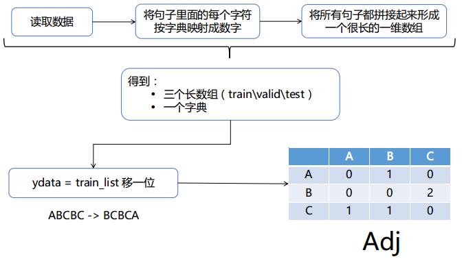
1. 将句子按字典映射成数字序列

1
2
3
for every sentences:
在句子后面加“|”(人为地添加句子的结束标识符)
将句子里面的*每个字符*映射成该字符在字典中*对应的数字*

例如:

p i e r r e < u n k > N y e a r s o l d w i l l j o i n t h e b o a r d a s a n o n e x e c u t i v e d i r e c t o r n o v . N |

[24, 10, 1, 2, 2, 1, 3, 27, 15, 5, 6, 28, 3, 29, 3, 14, 1, 0, 2, 16, 3, 7, 9, 21, 3, 13, 10, 9, 9, 3, 30, 7, 10, 5, 3, 8, 20, 1, 3, 4, 7, 0, 2, 21, 3, 0, 16, 3, 0, 3, 5, 7, 5, 1, 25, 1, 12, 15, 8, 10, 31, 1, 3, 21, 10, 2, 1, 12, 8, 7, 2, 3, 5, 7, 31, 32, 3, 29, 26]

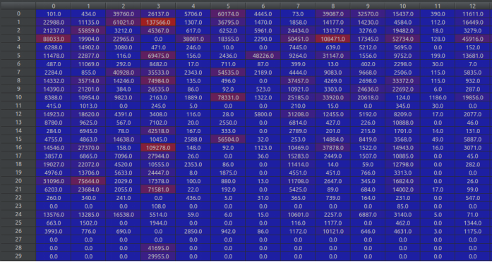
2. 构造邻接矩阵

得到邻接矩阵的值:

GCRN实现思路:

GCRN = GCN + RNN。

公式

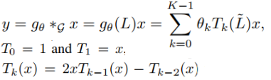
但是 代码中的实现方式稍有不同

GCN

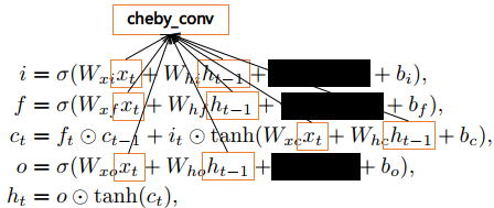
每次得到的 $T_k(x)$ 都与x做concat,最后得到的x与W相乘

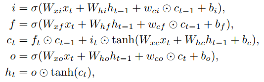
LSTM

开始训练

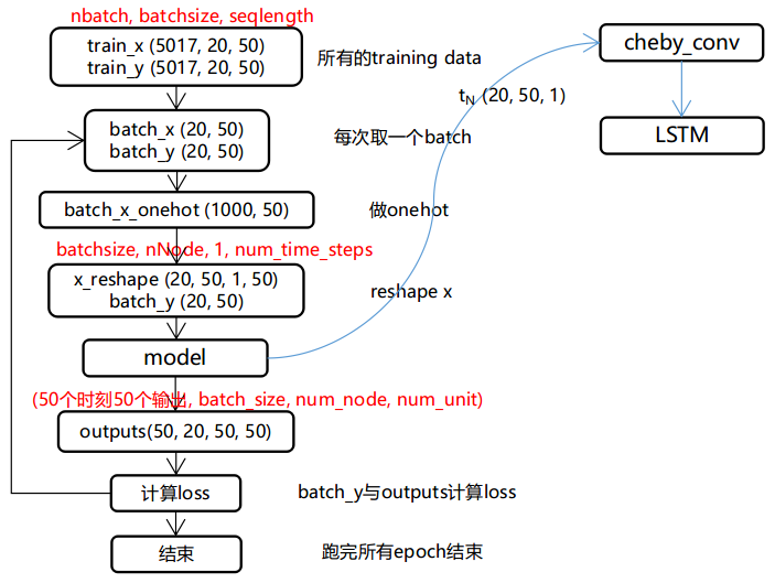
数据预处理 -> model定义 -> train

输出ouput的shape为(batch_size, num_node, num_unit) —— (20, 50, 50)。由于设置了有50个LSTM units,所以这里需要使所有units的输出做线性变换,使其变为一个值:

  • prediction = output * W -b,这里的prediction的shape为(20, 50, 1)

那么,所有时刻的输出的shape为(50, 20, 50, 1)

代码

GCN实现方法

1
2
3
4
5
6
7
8
9
10
11
12
13
14
15
16
17
18
19
20
21
22
23
24
25
26
27
28
29
30
31
32
33
34
35
36
37
38
39
40
41
42
43
44
45
def cheby_conv(x, L, lmax, feat_out, K, W):
'''
x : [batch_size, N_node, feat_in] - input of each time step
nSample : number of samples = batch_size
nNode : number of node in graph
feat_in : number of input feature
feat_out : number of output feature
L : laplacian
lmax : ?
K : size of kernel(number of cheby coefficients)
W : cheby_conv weight [K * feat_in, feat_out]
'''
nSample, nNode, feat_in = x.get_shape()
nSample, nNode, feat_in = int(nSample), int(nNode), int(feat_in)
L = graph.rescale_L(L, lmax) #What is this operation?? --> rescale Laplacian
L = L.tocoo()

indices = np.column_stack((L.row, L.col))
L = tf.SparseTensor(indices, L.data, L.shape)
L = tf.sparse_reorder(L)

x0 = tf.transpose(x, perm=[1, 2, 0]) #change it to [nNode, feat_in, nSample]
x0 = tf.reshape(x0, [nNode, feat_in*nSample])
x = tf.expand_dims(x0, 0) # make it [1, nNode, feat_in*nSample]

def concat(x, x_):
x_ = tf.expand_dims(x_, 0)
return tf.concat([x, x_], axis=0)

if K > 1:
x1 = tf.sparse_tensor_dense_matmul(L, x0)
x = concat(x, x1)

for k in range(2, K):
x2 = 2 * tf.sparse_tensor_dense_matmul(L, x1) - x0
x = concat(x, x2)
x0, x1 = x1, x2

x = tf.reshape(x, [K, nNode, feat_in, nSample])
x = tf.transpose(x, perm=[3,1,2,0])
x = tf.reshape(x, [nSample*nNode, feat_in*K])

x = tf.matmul(x, W) #No Bias term?? -> Yes
out = tf.reshape(x, [nSample, nNode, feat_out])
return out

LSTM实现方法

1
2
3
4
5
6
7
8
9
10
11
12
13
14
15
16
17
18
19
20
21
22
23
24
25
26
27
28
29
30
31
32
33
34
35
36
37
38
39
40
41
42
43
44
45
46
47
48
49
50
51
52
53
54
55
56
57
58
59
60
61
62
63
64
65
66
67
68
69
70
71
72
73
74
75
76
77
78
79
80
81
82
83
84
85
86
87
88
89
90
91
92
93
94
95
96
97
98
99
100
101
def __call__(self, inputs, state, scope=None):
with tf.variable_scope(scope or type(self).__name__):
if self._state_is_tuple:
c, h = state
else:
c, h = tf.split(value=state, num_or_size_splits=2, axis=1)
laplacian = self._laplacian
lmax = self._lmax
K = self._K
feat_in = self._feat_in

#The inputs : [batch_size, nNode, feat_in, nTime?] size tensor
if feat_in is None:
#Take out the shape of input
batch_size, nNode, feat_in = inputs.get_shape()
print("hey!")

feat_out = self._num_units

if K is None:
K = 2

scope = tf.get_variable_scope()
with tf.variable_scope(scope) as scope:
try:
#Need four diff Wconv weight + for Hidden weight
Wzxt = tf.get_variable("Wzxt", [K*feat_in, feat_out], dtype=tf.float32,
initializer=tf.random_uniform_initializer(minval=-0.1, maxval=0.1))
Wixt = tf.get_variable("Wixt", [K*feat_in, feat_out], dtype=tf.float32,
initializer=tf.random_uniform_initializer(minval=-0.1, maxval=0.1))
Wfxt = tf.get_variable("Wfxt", [K*feat_in, feat_out], dtype=tf.float32,
initializer=tf.random_uniform_initializer(minval=-0.1, maxval=0.1))
Woxt = tf.get_variable("Woxt", [K*feat_in, feat_out], dtype=tf.float32,
initializer=tf.random_uniform_initializer(minval=-0.1, maxval=0.1))

Wzht = tf.get_variable("Wzht", [K*feat_out, feat_out], dtype=tf.float32,
initializer=tf.random_uniform_initializer(minval=-0.1, maxval=0.1))
Wiht = tf.get_variable("Wiht", [K*feat_out, feat_out], dtype=tf.float32,
initializer=tf.random_uniform_initializer(minval=-0.1, maxval=0.1))
Wfht = tf.get_variable("Wfht", [K*feat_out, feat_out], dtype=tf.float32,
initializer=tf.random_uniform_initializer(minval=-0.1, maxval=0.1))
Woht = tf.get_variable("Woht", [K*feat_out, feat_out], dtype=tf.float32,
initializer=tf.random_uniform_initializer(minval=-0.1, maxval=0.1))
except ValueError:
scope.reuse_variables()
Wzxt = tf.get_variable("Wzxt", [K*feat_in, feat_out], dtype=tf.float32,
initializer=tf.random_uniform_initializer(minval=-0.1, maxval=0.1))
Wixt = tf.get_variable("Wixt", [K*feat_in, feat_out], dtype=tf.float32,
initializer=tf.random_uniform_initializer(minval=-0.1, maxval=0.1))
Wfxt = tf.get_variable("Wfxt", [K*feat_in, feat_out], dtype=tf.float32,
initializer=tf.random_uniform_initializer(minval=-0.1, maxval=0.1))
Woxt = tf.get_variable("Woxt", [K*feat_in, feat_out], dtype=tf.float32,
initializer=tf.random_uniform_initializer(minval=-0.1, maxval=0.1))

Wzht = tf.get_variable("Wzht", [K*feat_out, feat_out], dtype=tf.float32,
initializer=tf.random_uniform_initializer(minval=-0.1, maxval=0.1))
Wiht = tf.get_variable("Wiht", [K*feat_out, feat_out], dtype=tf.float32,
initializer=tf.random_uniform_initializer(minval=-0.1, maxval=0.1))
Wfht = tf.get_variable("Wfht", [K*feat_out, feat_out], dtype=tf.float32,
initializer=tf.random_uniform_initializer(minval=-0.1, maxval=0.1))
Woht = tf.get_variable("Woht", [K*feat_out, feat_out], dtype=tf.float32,
initializer=tf.random_uniform_initializer(minval=-0.1, maxval=0.1))


bzt = tf.get_variable("bzt", [feat_out])
bit = tf.get_variable("bit", [feat_out])
bft = tf.get_variable("bft", [feat_out])
bot = tf.get_variable("bot", [feat_out])

# gconv Calculation
zxt = cheby_conv(inputs, laplacian, lmax, feat_out, K, Wzxt)
zht = cheby_conv(h, laplacian, lmax, feat_out, K, Wzht)
zt = zxt + zht + bzt
zt = tf.tanh(zt)

ixt = cheby_conv(inputs, laplacian, lmax, feat_out, K, Wixt)
iht = cheby_conv(h, laplacian, lmax, feat_out, K, Wiht)
it = ixt + iht + bit
it = tf.sigmoid(it)

fxt = cheby_conv(inputs, laplacian, lmax, feat_out, K, Wfxt)
fht = cheby_conv(h, laplacian, lmax, feat_out, K, Wfht)
ft = fxt + fht + bft
ft = tf.sigmoid(ft)

oxt = cheby_conv(inputs, laplacian, lmax, feat_out, K, Woxt)
oht = cheby_conv(h, laplacian, lmax, feat_out, K, Woht)
ot = oxt + oht + bot
ot = tf.sigmoid(ot)

# c
new_c = ft*c + it*zt

# h
new_h = ot*tf.tanh(new_c)

if self._state_is_tuple:
new_state = LSTMStateTuple(new_c, new_h)
else:
new_state = tf.concat([new_c, new_h], 1)
return new_h, new_state

其他变量

变量 shape meaning
rnn_input (20, 50, 1, 50) (batch_size, num_node, feat_in, num_time_steps)
rnn_input_seq (20, 50, 1) * 50 (batch_size, num_node, feat_in) * num_time_steps
rnn_output (20, 50) (batch_size, num_time_steps)
rnn_output_seq (20) * 50 (batch_size) * num_time_steps
num_hidden 50 隐藏层单元
x_batches (5017, 20, 50) [-1, batch_size, seq_length]
y_batches (5017, 20, 50) [-1, batch_size, seq_length]
outputs (50, 20, 50, 50) (50个时刻50个输出, batch_size, num_node, num_unit)
output (20, 50, 50) outputs的单个时刻输出(batch_size, num_node, num_unit)

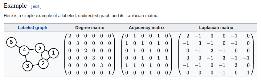
Laplacian matrix

Properties

对一个无向图$G$和他的laplacian matrix $L$,有特征值$\lambda_0 \leq \lambda_1 \leq \lambda_2 …$:

  • L是对称的
  • L是半正定的(即所有$\lambda_i > 0$),这可以在关联矩阵部分验证,也同样可以从Laplacian是对称并且对角占优(diagonally dominant)得出
  • L是M-matrix(它的非对角线上的项是负的,但它的特征值的实部为负)
  • 行或列相加结果为0
  • L的最小非零特征值称为谱间隙(spectral gap)
  • 图中连通分量的个数是拉普拉斯算子的零空间维数和0特征值的代数多重性
  • 拉普拉斯矩阵是奇异的

问题

  1. 代码实现里面的公式跟论文是否真的不一样
  2. x2 = 2 * tf.sparse_tensor_dense_matmul(L, x1) - x0 起到一个什么作用

后记

补充一下,后来跟实验室的小伙伴谈论过后对GCN有了比较深刻的认识。上面问题中的第二点,其实跟GCN的K的大小有关。K=1,表示包含了该节点一条的信息。至于为什么会这样,这是因为在计算过程中与由adj mnatrix得来的Laplacian相乘,每乘一次,就会多包含一跳的节点信息。

Sparse matrix

稀疏矩阵指的是矩阵里面的元素大多都是0值。

与 sparse 相对的,就是 dense, which most elements of the matrix are nonzero

矩阵的稀疏性 = zero-valued elements / total number of elements

Sparse Representation

Q:稀疏表达有什么好处?

稀疏表达的意义在于降维,但是我还是不知道这个怎么搞得

Q:稀疏表达 sparse representation 与 降维 dimensionality reduction 本质区别在哪?

降维是将原 space 里的数据在某一个 subspace 里面表达,而稀疏表达是在 a union subspace 里面表达。

举个例子

(x, y, z)的空间中,(x, y)就是其中一个 subspace 。而 a union subspace 就包含了多个 subspace ,比如[(x, y), (y, z), (z, x)]就是 a union subspace。

Q:如何求得数据的稀疏矩阵?

to be continue

Storing a sparse matrix

Compressed sparse row(CSR, CRS pr Yale format)

```python # data A = data = (5, 8, 3, 6) # indptr的第一个元素为0,数值表示共有多少非零元素 IA = indptr = (0, 0, 2, 3, 4) # 每个data的index JA = indices = (0, 1, 2, 1)
1
2
3
4
5
6
7
8
9
10
11
<script type="math/tex; mode=display">
MatrixB =
\begin{pmatrix}
10 & 20 & 0 & 0 & 0 & 0 \\
0 & 30 & 0 & 40 & 0 & 0 \\
0 & 0 & 50 & 60 & 70 & 0 \\
0 & 0 & 0 & 0 & 0 & 80 \\
\end{pmatrix}</script>```python
A = data = (10, 20, 30, 40, 50, 60, 70, 80)
IA = indptr = (0, 2, 4, 7, 8)
JA = indices = (0, 1, 1, 3, 2, 3, 4, 5)

List of list(LIL)

LIL stores one list per row, with each entry containing the column index and the value. Typically, these entries are kept sorted by column index for faster lookup. This is another format good for incremental matrix construction.

1
2
3
4
5
6
7
8
9
10
11
12
13
14
15
16
17
MatrixA:

(1, 0) 5
(1, 1) 8
(2, 2) 3
(1, 1) 6

MatrixB:

(0, 0) 10
(0, 1) 20
(1, 1) 30
(1, 3) 40
(2, 2) 50
(2, 3) 60
(2, 4) 70
(3, 5) 80

例子:这里


参考:
https://www.zhihu.com/question/26602796/answer/33431062
https://www.zhihu.com/question/24124122/answer/50403932
https://en.wikipedia.org/wiki/Sparse_matrix

0%